
Artificial Intelligence is transforming the cybersecurity landscape by offering advanced techniques to identify and mitigate emerging threats. As cyberattacks grow more sophisticated, AI is increasingly relied upon to strengthen security frameworks. A promising area where AI shines is in detecting Distributed Denial of Service (DDoS) attacks. These attacks flood networks with malicious traffic, disrupting services and causing serious harm to businesses and infrastructure. Traditional DDoS detection methods often struggle with the scale and complexity of modern attacks, but AI presents a powerful solution.
Using machine learning algorithms and pattern recognition, AI can analyze massive amounts of network traffic data in real-time, spotting anomalies that might signal a DDoS attack. Its ability to continuously learn from new data means AI can evolve in response to the shifting tactics of cybercriminals. Furthermore, AI-driven systems can respond faster than manual methods, providing early warnings and automating defensive measures.
In this project, I’m diving into the process of machine learning. Part I Agenda
- Project Goals
- What does the process look like?
- Dataset
- Environment
- Data Exploration
- Coclusion
Project Goals
As the title suggests, the main goal of this project is to detect DDoS attacks using AI techniques. But, as a complete newbie to the topic, I know this journey will be about much more than that. My goal is to understand the process and apply theoretical knowledge in a hands-on project. Sounds simple, but I’m ready for things to get complex… What Does the Process Look Like?
Process of what, exactly?
From here on, I’ll use the term Machine Learning (ML) since my project requires training an algorithm on data to build a model that can make predictive decisions—in this case, answering the simple question, “Is it DDoS?”
So, what does the process of Machine Learning look like? I love the diagram prepared by the authors of the excellent book Machine Learning with PyTorch and Scikit-Learn by Sebastian Raschka, Yuxi (Hayden) Liu, and Vahid Mirjalili.
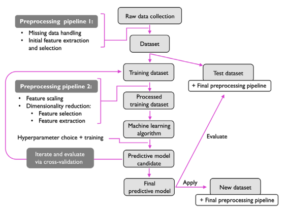
I’m not going to describe every single step. It’s not my intention to overwhelm you with a huge amount of information. Instead, I’d rather explain it alongside the implementation of each step. Hope you’re okay with that (if not, I don’t care—it’s my blog!).
For now, this picture should be sufficient to give you a broad overview of the process.
Dataset
I’m pretty sure that if you asked anyone, “What’s the most important aspect of Machine Learning?” the answer would always be the same: D A T A. Don’t have enough data? Fail. Your data lacks crucial information? Fail. Data isn’t clean enough? Faiiiiiil.
The entire process is based on data and the associated processes: cleaning, feature extraction, standardization, labeling (for supervised learning), splitting, training, testing, evaluating, and so on. It all starts with gathering data. Luckily, I’ve been equipped with the CICDDoS2019 dataset.
CICDDoS2019 contains benign data and the most up-to-date common DDoS attacks, resembling real-world data (PCAPs). It also includes results from network traffic analysis using CICFlowMeter-V3, which labels flows based on timestamps, source and destination IPs, source and destination ports, protocols, and attacks (in CSV format). Generating realistic background traffic was our top priority when building this dataset. We used our proposed B-Profile system (Sharafaldin et al., 2016) to profile the abstract behavior of human interactions and generate naturalistic benign background traffic in the proposed testbed (see Figure 2). For this dataset, we constructed the abstract behavior of 25 users based on HTTP, HTTPS, FTP, SSH, and email protocols.
Those packages are heavy—I’m talking about gigabytes of pure data in CSV format!
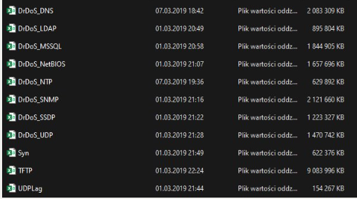
“In this dataset, we have different modern reflective DDoS attacks such as PortMap, NetBIOS, LDAP, MSSQL, UDP, UDP-Lag, SYN, NTP, DNS and SNMP. Attacks were subsequently executed during this period. (…) we executed 12 DDoS attacks includes NTP, DNS, LDAP, MSSQL, NetBIOS, SNMP, SSDP, UDP, UDP-Lag, WebDDoS, SYN and TFTP on the training day and 7 attacks including PortScan, NetBIOS, LDAP, MSSQL, UDP, UDP-Lag and SYN in the testing day. The traffic volume for WebDDoS was so low and PortScan just has been executed in the testing day and will be unknown for evaluating the proposed model.”
For my project purpose I will focus on just one chunk of dataset - DrDoS_DNS. I’m not going to let this project overwhelm me, thus, I’ve decided to pick just one and learn the process. Let’s set up the environment and finally get started.
Environment
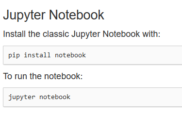
Jupyter is the most frequently chosen environment. As we all stand on the shoulders of giants I’m not gonna question this choice (for now). Another advantage is that to set it all up, we just need few commands, and to be more precise - two of them:
I’m aware that this project may need some Python libraries so to avoid any incompatibility I’ll just use virtual envirnonment. venv module is lightweight and can help me isolate my project so it sounds like a perfect choice.
python3 -m venv [name of the virtual envirnment]source [name]/bin/activateAfter activating the virtual environment I’m just ready to run my notebook.
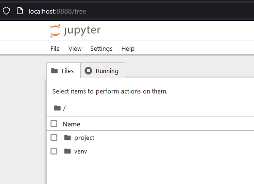
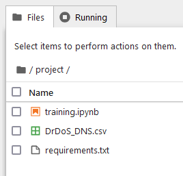
As you can see I named my virtual environment as venv. Not so creative but works anyway. This project folder is the place where I store my chunky csv file.
-
training.ipynb - text-based file used by Jupyter Notebook - a web-based interactive computing programme that helps users analyse and manipulate data using the Python programming language.
-
DrDos_DNS.csv - file with logs/packets
-
requirements.txt - file with all the libraries that might be useful, in Python project they can be installed collectively using
pip install -r requirements.txtFor now it doesn’t matter what’s in there.
That’s all regarding the environment. From now on I will focus on jupyter file (training.ipynb) where I will be learning the process.
Data exploration
We can finally take a look at our csv file. Jupyter is a tool that supports interactive data science and scientific computing across all programming languages. Meaning you don’t need to write the whole code, compile it and then run. We are working with blocks of code, just take a look:
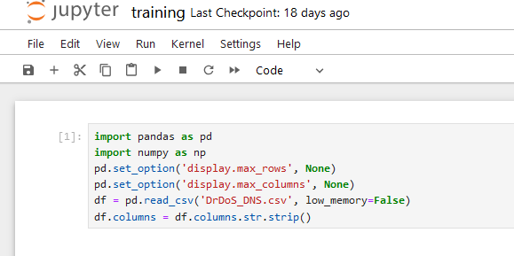
This is our first block, keep in mind that each line could be divided into separate block. I like to think about it in frames of one action=one block. Just like the proper function should be written. So, that block is the “defining block”. We import libraries and defining which data we are gonna work on.
These lines in Python are doing the following:
-
import pandas as pd
This imports thepandaslibrary and assigns it the shorthand aliaspd.pandasis a library commonly used for data analysis and manipulation in Python. -
import numpy as np
This imports thenumpylibrary, also with a shorthand alias (np).numpyis used for working with arrays and provides mathematical functions needed for scientific computations. -
pd.set_option('display.max_rows', None)
This line configurespandasto display all rows when showing data in the console (by default,pandaslimits the number of rows displayed). Setting this toNoneremoves that limit. -
pd.set_option('display.max_columns', None)
Similar to the line above, this configurespandasto display all columns when displaying a DataFrame. Without this,pandasmight cut off columns when displaying wide tables. -
df = pd.read_csv('DrDoS_DNS.csv', low_memory=False)
This reads a CSV file named'DrDoS_DNS.csv'into aDataFramecalleddf. Thelow_memory=Falseoption loads the entire file at once, avoiding data type guessing that might happen with larger files. Settinglow_memory=Falsecan prevent certain types of warnings, especially with large datasets. -
df.columns = df.columns.str.strip()
This line removes any leading or trailing whitespace from the column names indf. This is particularly useful if the column names accidentally have extra spaces that could interfere with accessing them correctly in the code.
With that block we are ready to start messing around with the data.
Features
In machine learning, features are the individual measurable properties or characteristics of the data used to make predictions or classifications. Each feature represents a specific aspect of the data, and collectively, features provide the model with the information it needs to learn patterns and make accurate predictions.
Let’s find out what features do we got by using below command:
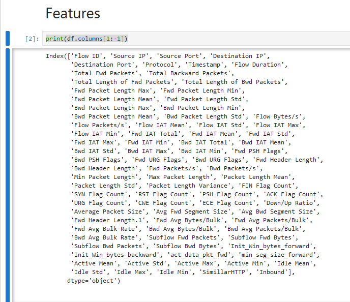
The line print(df.columns[1:-1]) prints a subset of the column names in a DataFrame, specifically all columns except the first and last. What’s wrong with first and the last? Let me show you:
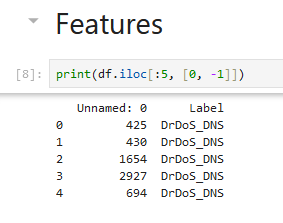
That command prints first 5 rows of the first and last columns. Label column is just label, not a feature, and the first one is like an index so it doesn’t provide any valuable info.
We’ve printed out our features but how many do we got? I ain’t gonna count them but I know the command that can do it for me:
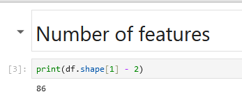
It calculates the number of columns in the DataFrame df minus 2 (first and last), and then prints the result. So, we got 86 features which is quite decent.
Observations
But how many packets do we got?
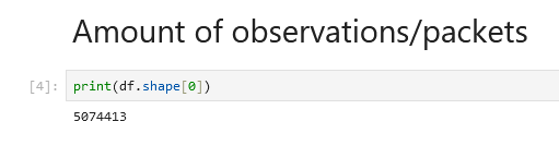
It prints the number of rows in the DataFrame df. Oh man,
5,074,413 rows. Over 5 million packets. That’s a lot.
Labels
Distribiution (or ratio) of labels might be the most crucial aspect of this dataset. Balance is the key. But first, let’s find out what names of labels do we have?
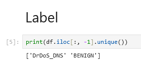
Fine, will work. It could be translated as “DDoS traffic” and “No DDoS traffic”. Okay, it’s time for distribuition:
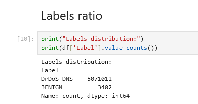
Oh man, that’s imbalanced as hell. I will need to figure out what to do with that later.
Vector Example
Using random column I wanted to see how does the column look like. print(df.iloc[131]) should do the work:
Unnamed: 0 928Flow ID 172.16.0.5-192.168.50.1-634-51124-17Source IP 172.16.0.5Source Port 634Destination IP 192.168.50.1Destination Port 51124Protocol 17Timestamp 2018-12-01 10:51:43.900176Flow Duration 47202Total Fwd Packets 200Total Backward Packets 0Total Length of Fwd Packets 88000.0Total Length of Bwd Packets 0.0Fwd Packet Length Max 440.0Fwd Packet Length Min 440.0Fwd Packet Length Mean 440.0Fwd Packet Length Std 0.0Bwd Packet Length Max 0.0Bwd Packet Length Min 0.0Bwd Packet Length Mean 0.0Bwd Packet Length Std 0.0Flow Bytes/s 1864327.782721Flow Packets/s 4237.108597Flow IAT Mean 237.19598Flow IAT Std 337.199588Flow IAT Max 2016.0Flow IAT Min 1.0Fwd IAT Total 47202.0Fwd IAT Mean 237.19598Fwd IAT Std 337.199588Fwd IAT Max 2016.0Fwd IAT Min 1.0Bwd IAT Total 0.0Bwd IAT Mean 0.0Bwd IAT Std 0.0Bwd IAT Max 0.0Bwd IAT Min 0.0Fwd PSH Flags 0Bwd PSH Flags 0Fwd URG Flags 0Bwd URG Flags 0Fwd Header Length 6400Bwd Header Length 0Fwd Packets/s 4237.108597Bwd Packets/s 0.0Min Packet Length 440.0Max Packet Length 440.0Packet Length Mean 440.0Packet Length Std 0.0Packet Length Variance 0.0FIN Flag Count 0SYN Flag Count 0RST Flag Count 0PSH Flag Count 0ACK Flag Count 0URG Flag Count 0CWE Flag Count 0ECE Flag Count 0Down/Up Ratio 0.0Average Packet Size 442.2Avg Fwd Segment Size 440.0Avg Bwd Segment Size 0.0Fwd Header Length.1 6400Fwd Avg Bytes/Bulk 0Fwd Avg Packets/Bulk 0Fwd Avg Bulk Rate 0Bwd Avg Bytes/Bulk 0Bwd Avg Packets/Bulk 0Bwd Avg Bulk Rate 0Subflow Fwd Packets 200Subflow Fwd Bytes 88000Subflow Bwd Packets 0Subflow Bwd Bytes 0Init_Win_bytes_forward -1Init_Win_bytes_backward -1act_data_pkt_fwd 199min_seg_size_forward 32Active Mean 0.0Active Std 0.0Active Max 0.0Active Min 0.0Idle Mean 0.0Idle Std 0.0Idle Max 0.0Idle Min 0.0SimillarHTTP 0Inbound 1Label DrDoS_DNSName: 131, dtype: objectMany 0s… it doesn’t seem promising. But we will worry about that later.
Types of data
To check out the types of data I used df.info():
<class 'pandas.core.frame.DataFrame'>RangeIndex: 5074413 entries, 0 to 5074412Data columns (total 88 columns): # Column Dtype--- ------ ----- 0 Unnamed: 0 int64 1 Flow ID object 2 Source IP object 3 Source Port int64 4 Destination IP object 5 Destination Port int64 6 Protocol int64 7 Timestamp object 8 Flow Duration int64 9 Total Fwd Packets int64 10 Total Backward Packets int64 11 Total Length of Fwd Packets float64 12 Total Length of Bwd Packets float64 13 Fwd Packet Length Max float64 14 Fwd Packet Length Min float64 15 Fwd Packet Length Mean float64 16 Fwd Packet Length Std float64 17 Bwd Packet Length Max float64 18 Bwd Packet Length Min float64 19 Bwd Packet Length Mean float64 20 Bwd Packet Length Std float64 21 Flow Bytes/s float64 22 Flow Packets/s float64 23 Flow IAT Mean float64 24 Flow IAT Std float64 25 Flow IAT Max float64 26 Flow IAT Min float64 27 Fwd IAT Total float64 28 Fwd IAT Mean float64 29 Fwd IAT Std float64 30 Fwd IAT Max float64 31 Fwd IAT Min float64 32 Bwd IAT Total float64 33 Bwd IAT Mean float64 34 Bwd IAT Std float64 35 Bwd IAT Max float64 36 Bwd IAT Min float64 37 Fwd PSH Flags int64 38 Bwd PSH Flags int64 39 Fwd URG Flags int64 40 Bwd URG Flags int64 41 Fwd Header Length int64 42 Bwd Header Length int64 43 Fwd Packets/s float64 44 Bwd Packets/s float64 45 Min Packet Length float64 46 Max Packet Length float64 47 Packet Length Mean float64 48 Packet Length Std float64 49 Packet Length Variance float64 50 FIN Flag Count int64 51 SYN Flag Count int64 52 RST Flag Count int64 53 PSH Flag Count int64 54 ACK Flag Count int64 55 URG Flag Count int64 56 CWE Flag Count int64 57 ECE Flag Count int64 58 Down/Up Ratio float64 59 Average Packet Size float64 60 Avg Fwd Segment Size float64 61 Avg Bwd Segment Size float64 62 Fwd Header Length.1 int64 63 Fwd Avg Bytes/Bulk int64 64 Fwd Avg Packets/Bulk int64 65 Fwd Avg Bulk Rate int64 66 Bwd Avg Bytes/Bulk int64 67 Bwd Avg Packets/Bulk int64 68 Bwd Avg Bulk Rate int64 69 Subflow Fwd Packets int64 70 Subflow Fwd Bytes int64 71 Subflow Bwd Packets int64 72 Subflow Bwd Bytes int64 73 Init_Win_bytes_forward int64 74 Init_Win_bytes_backward int64 75 act_data_pkt_fwd int64 76 min_seg_size_forward int64 77 Active Mean float64 78 Active Std float64 79 Active Max float64 80 Active Min float64 81 Idle Mean float64 82 Idle Std float64 83 Idle Max float64 84 Idle Min float64 85 SimillarHTTP object 86 Inbound int64 87 Label objectdtypes: float64(45), int64(37), object(6)memory usage: 3.3+ GBConclusion
I can’t complain about the lack of variety of data but I can see that there’s much to do with cleaning stuff. I will devote next chapter to data cleaning. I will focus on handling missing data, removing vectors and then making hard decsion on choosing the right features. But that’s just tomorrow me problem. Hope you enjoyed the first episode. Check out for next
~Type